Investors always want to earn as much average (mean) return as possible with as little volatility as possible, but in general, more return comes with more volatility. Investing is all about deciding what an appropriate risk level is and then getting as much return as possible while only taking the appropriate amount of risk. There are two components to differentiating risk-adjusted returns versus a benchmark. The first component is the weighted average risk-adjusted return of the investments in the portfolio. The Retirement Group absolutely attempts to select investments that subsequently earn better risk-adjusted returns than the portfolio’s benchmark, as it should. The challenge with this part of the approach is that it typically comes with a compromise in liquidity or a requirement the manager of the investment has some exceptional level of skill that will likely persist in the future.
As long as the liquidity of the entire portfolio is managed appropriately, having some illiquidity within a portfolio is not problematic. With regards to evaluating the skill of a manager, The Retirement Group does go well beyond just evaluating the past performance of a manager when assessing a third party manager’s skill to mitigate the risk of finding managers who have simply been lucky in the past and are unlikely to see their strong historical performance continue into the future. This paper, however, focuses on a different component to risk-adjusted performance at the portfolio level that does not require that the underlying investments have risk-adjusted performance that is superior to that of the portfolio’s benchmark. This aspect of what The Retirement Group does is called diversification. Diversification does not by itself increase a portfolio’s mean return, but it does reduce a portfolio’s volatility. By volatility, I mean the standard deviation of returns. Standard deviation is a measure of the degree to which returns typically deviate from their average. A low standard deviation means that most annual returns are very close to the average return. A high standard deviation means that it is not uncommon for an annual return to be significantly higher or significantly lower than the average. Typically in investing, asset classes with higher standard deviations also have higher mean returns. Stocks, for example, tend to have a higher level of standard deviation than bonds and are thus viewed as riskier than bonds. As compensation for taking that extra risk, investors in stocks are typically rewarded with higher mean returns over time. Diversification offers investors a way to reduce portfolio standard deviation without reducing portfolio mean return.
The secret to this trick is a correlation. Correlation is a statistical measure of the degree to which two data series (in this case returns to two different asset classes) move together. Correlation ranges between -1 and 1. A correlation of -1 means the worst returns for one asset class occur at the same time as the best returns for the other asset class, mediocre returns for one asset class occur at the same time as pretty good returns for the other asset class, and average returns for both asset classes occur at the same time. A correlation of 1 means that the best returns for the first asset class occur at exactly the same time as the best returns for the second asset class, the worst returns for the first asset class occur at exactly the same time as the worst returns for the second asset class, and average returns for both asset classes occur at the same time. A correlation of 0 means that the returns of the first asset class tell you nothing about what the returns of the second asset class likely were. A simple example may help illustrate how diversification works. Chart 1 shows the performance of two assets, Asset A and Asset B, and the performance of a portfolio that allocates equally to both assets with continuous rebalancing. Asset A delivers a return of 25% in the first year and Asset B delivers a return of -5% in the first year. In the second year, Asset A is -5% and Asset B is 25%.
This two-year cycle repeats itself five times, so ultimately Asset A and Asset B grow from a $100 investment to $236.14 over the course of ten years, meaning both Asset A and Asset B deliver an 8.97% return per year. The equal-weighted portfolio also grows by $100 to $236.14 over ten years, so its annualized mean return is also 8.97%. In this example, mean returns are clearly unaffected by diversification. Volatility, on the other hand, is significantly impacted by diversification. Imagine if the portfolio were just 100% allocated to Asset A or to Asset B. In some years the portfolio would be up 25% and in other years it would be down -5%. The annualized standard deviation would be 14.46% for either Asset A or Asset B as stand-alone portfolios. This would be a much less comfortable experience than the equal-weighted portfolio would provide. The equal-weighted portfolio would be up 8.97% every year with an annualized standard deviation of 0%. There would be no really big up years and no down years. The reason there is no volatility in the equal-weighted portfolio is that every time one asset has a bad year, that bad year is offset by a good year from the other asset. In the real world, things are not quite this simple. There are more than two assets and the returns are less predictable and not perfectly negatively correlated with each other. The concept still works in the real world though. Diversifying may not eliminate volatility entirely like in Chart 1’s example, but it does reduce it.

WARNING: For those readers who are math lovers will enjoy seeing how the mathematics of diversification works in the next few paragraphs, but those who are less quantitatively inclined may want to just skim this section and then skip down to the section titled “An Extreme Example.”


The neat thing about diversification is that it does not require a compromise on liquidity and it does not require the investor to be an expert at predicting the future. As long as correlations between asset classes are less than perfectly positive and there are several asset classes in the portfolio, risk can be reduced significantly without reducing mean return. As an extreme example, assume you have a portfolio with 100 different asset classes. Every asset class has an expected return of 10% per year and a standard deviation of 24% per year. As an aside, these are White Oaks' prospective assumptions for emerging market stocks, so this portfolio has 100 different asset classes that all have the risk and return profiles of emerging market stocks. This portfolio is clearly allocated exclusively to investments that would be considered by most investors to be very risky.
Of course, if we assume these 100 asset classes are all completely uncorrelated to each other, something very interesting happens. This portfolio, which is invested exclusively in very risky investments, only has an annualized standard deviation of 2.4%. For reference, White Oaks is currently assuming an annualized standard deviation of 3% for bonds, which most investors would consider to be conservative. Through the magic of diversification, a portfolio that only has investments with emerging markets equities’ type risk has less than bond-like risk because it is extremely well diversified.
Of course, the bond investor is likely to earn much lower portfolio mean returns (The White Oaks currently assumes 2.5%) than the 100-asset investor, whose portfolio mean return is 10%. The reason the 100-asset investor can reasonably expect higher mean returns is because he is taking more risk with each investment and is being compensated for that additional risk with the more expected return, but at the portfolio level most of that risk is being diversified away. To assume that investments with more volatility do not generally offer higher mean returns is to make an assumption about differences in the Sharpe Ratio across different asset classes, which is a different part of the decomposition of portfolio risk-adjusted returns. This 100-asset investor gets emerging equity type mean returns at bond-like risk by fully exploiting the power of diversification.
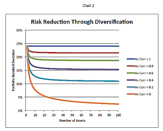
Chart 2 shows the portfolio standard deviation of other portfolios that exclusively invest in assets with standard deviations of 24% per year and shows varying numbers of investments and average correlations between those investments. Zero correlation and 100 hundred assets take annualized portfolio standard deviation from 24% to 2.40%. Even a 0.4 correlation and only ten assets take annualized portfolio standard deviation from 24% to 16.28%. With a zero correlation and five assets, annualized portfolio standard deviation goes from 24% to 10.73%.
Chart 2 gives a nice illustration of how much more effective diversification is when correlations are lower.